How sure should the bike plan be?
Turning one-day Citi Bike forecasts into decisions under uncertainty — why raw quantile bands lied, how conformalization restored 80% coverage, and when the 90th percentile becomes the truck plan.
Every night, Citi Bike's rebalancing trucks move bikes to where tomorrow's riders will want them. Over-forecast a station and you waste truck-hours; under-forecast and a commuter finds an empty dock at 8 am. A point forecast can tell the planner what is likely. It cannot answer the operational question by itself: how many bikes should we stage if being short is much worse than being long?
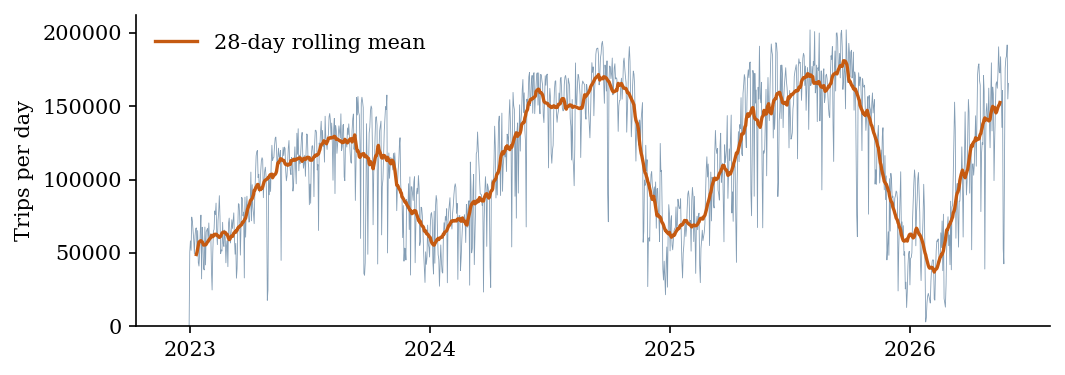
The raw material: every trip the system recorded from January 2023 through May 2026 — 139.6 million trips across ~2,200 stations — plus NOAA daily weather. Twenty gigabytes of raw files, aggregated month-by-month down to a few hundred megabytes of station-day counts before modeling ever started. The companion audit asks which model should own which horizon; this page asks what happens next, when a one-day forecast has to become a decision under uncertainty.
First, a forecast worth calibrating
The comparison set was fixed before any results were computed: a seasonal-naïve baseline ("same as last Friday"), a ridge regression on calendar and weather features, and LightGBM with lags and rolling levels. Each rung earns its place only by beating the rung below on the same backtest — twelve monthly folds covering June 2025 to May 2026, every model refit on strictly prior data. No random splits: with autocorrelated data, a random test day is surrounded in training by its own near-duplicates, and the backtest becomes fiction.
| Model | Station MAE (trips/day) | Skill vs. naïve |
|---|---|---|
| Seasonal naïve | 77.8 | — |
| Ridge regression | 48.0 | +38% |
| LightGBM | 38.6 | +50% |
The two failures worth more than the wins
Scale pooling. My first run pooled the citywide total (~110,000 trips/day) and individual stations (~300/day) into one linear fit. Squared loss let the big series dominate the coefficients, and station error came out 2.8× worse than the naïve baseline. The model wasn't broken — the pooling was.
Trees can't extrapolate. A regression tree predicts an average of what it has seen; it cannot forecast above its training range. With ridership growing every year, the tree model systematically under-forecast — until the target became the ratio of tomorrow to the station's trailing 28-day level. The level comes from the data; the model only predicts "how unusual will tomorrow be." That single change took skill from +5.7% to +50%. It's the tabular-ML analogue of differencing a time series, and it was the most consequential decision in the project.
Intervals that mean what they say
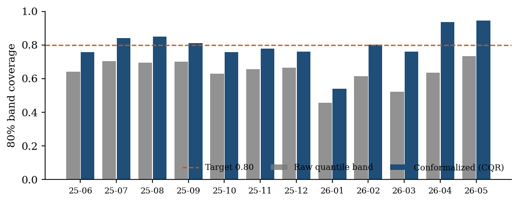
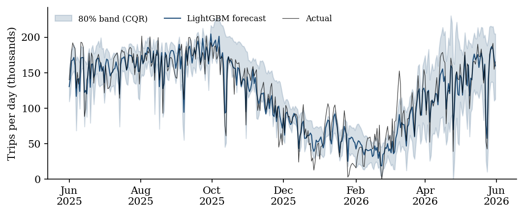
A point forecast can't drive a stocking decision — the truck plan needs "how bad might it get." Quantile-loss LightGBM produced 10th/50th/90th percentile forecasts, but the raw 80% band covered only 64% of actual outcomes: confidently wrong. Rather than hand-tune, conformalized quantile regression widens the band by exactly the margin that restores coverage on a held-out calibration window. Result: 79.5% coverage against an 80% target, stable across months. The honest band is ~43% wider than the overconfident one — that's not a cost, that's the truth surfacing.
Why the 90th percentile matters: if a stranded rider costs ~9× an idle truck-slot, the newsvendor rule says the optimal plan covers exactly the 90th percentile of demand. The quantile forecast is the staffing decision — which is what the one-page ops memo demonstrates on a real day (forecast 171.3k trips; actual 172.5k).
What this page leaves to the audit
The broader model-selection story — weather features, station granularity, horizon handoffs, and why simple baselines win farther out — belongs in the companion audit. Here LightGBM is the working forecast generator. The distinctive question is how to wrap that forecast in calibrated uncertainty and choose the quantile that matches the operating cost of being wrong.
What's disclosed, not buried
- The backtest uses realized weather as a stand-in for a day-ahead forecast, so reported skill is an upper bound on deployable skill.
- Observed trips are demand censored by supply: an empty dock records zero departures no matter how many riders walked away.
- The median forecast runs slightly low during steep seasonal ramps (June/November/March), where a trailing 28-day level lags — the noted next iteration is a ramp-aware level estimate.
The companion audit asks which forecast should own which decision horizon. This page asks how a one-day forecast becomes an operational decision once uncertainty and asymmetric costs are visible. The one-page decision layer is the ops memo (PDF).